GAMES202 Lecture 04 - Real-Time Shadows 2

GAMES202_Lecture_04 (ucsb.edu)

I. More on PCF and PCSS

The Principle behind PCF/PCSS

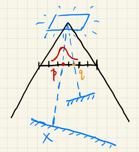
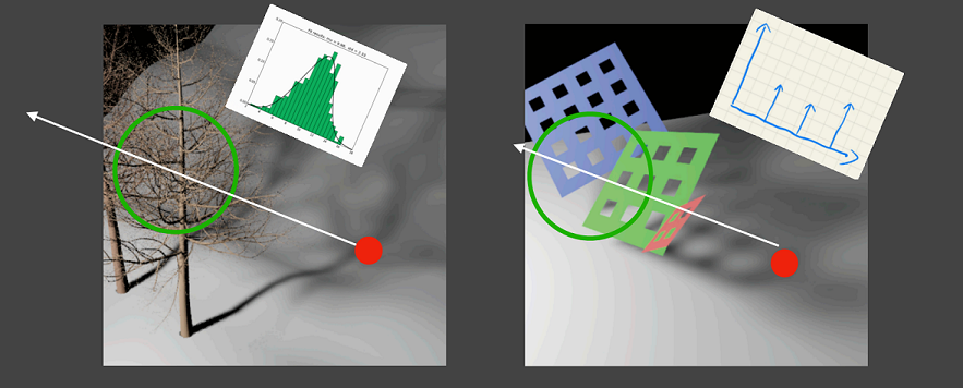
• Consider the Neighboring Region: For any point $x$$x$ being rendered, we consider the neighboring region of the corresponding texel $p$$p$ on the shadow map.

  • Weighted Consideration: When we average the entire region with all weights set to $1$$1$, then it is the traditional PCF/PCSS. We may also assign more weight to texels closer to $p$$p$, thus forming a weight distribution.

  • Filter/Convolution: Averaging w.r.t. to a specific distribution is essentially filter/convolution.

    $$[w\ast f](p)=\sum _{q\in \mathcal{N}(p)}w(p,q)f(q)$$

    where:

    • $w(p,q)$$w(p, q)$ represents weight when considering texel $q$$q$ in terms of $p$$p$, or the distribution,

    • $\mathcal{N}(p)$$\mathcal{N}(p)$ represents the neighboring region of point $p$$p$,

    • $f(x)$$f(x)$ is the function the convolution is done on, and

    • $[w\ast f]$$[w \ast f]$ is the result of convolution.

In PCSS:

For any shading point $x$$x$ which have its corresponding texel $p$$p$ on the shadow map, we consider the neighboring region of $p$$p$.

• For any texel $q$$q$ inside $\mathcal{N}(p)$$\mathcal{N}(p)$, we consider whether $x$$x$ will be blocked by $q$$q$.

• $V(x)$$V(x)$: the visibility of point $x$$x$

• ${\chi }^{+}$$\chi^+$: the sign function. If $t>0$$t > 0$, then ${\chi }^{+}(t)=1$$\chi^+(t) = 1$. Else, ${\chi }^{+}(t)=0$$\chi^+(t) = 0$.

Thus, we have the following conclusions:

• PCF is not filtering the shadow map and then comparing:

  $$V(x)\ne {\chi }^{+}\{[w\ast D_{\text{SM}}](q)-D_{\text{Scene}}(x)\}$$

  • Which still leads to binary visibilities

• PCF is not filtering the resulting image with binary visibilities:

  $$V(x)\ne \sum _{y\in \mathcal{N}(x)}w(x,y)V(y)$$

  • In other words, PCF is not filtering the resultant shadow.

Performance Issue in PCSS

Given the PCSS algorithm:

1. Blocker Search:

   • Get the average blocker depth in a certain region inside the shadow map

2. Penumbra Estimation:

   • Use the average blocker depth to determine filter size

3. Percentage Closer Filtering

Which steps can be slow in PCSS?

• Examining every texel in a certain region (steps 1 and 3)

  • Sample:

    • May use sparse sampling, and then apply image-space denoising.

    • Introducing noise.

  • MIPMAP

• Softer -> Larger Filtering Region -> Slower

II. Variance (Soft) Shadow Mapping (VSM/VSMM)

What is new in VSM/VSMM:

• Fast blocker search (step 1) and filtering (step 3) [Yang et al.]

Speeding up PCF

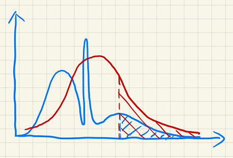
Predict the percentage of texels that are in front of the shading point:

• Using a normal distribution to approximate the answer

• Or, we may directly apply Chebyshev's inequality without assuming the distribution

Key Idea

Using probability theories to approximate the answer.

• Quickly compute the mean and variance of depths in an area

• Mean (Average):

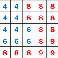
  • Hardware MIPMAP (Range-Average Query)

  • Summed Area Tables (SAT)

    • How to? See Section III.

• Variance:

  $$\text{Var}(X)=E(X^2)-E^2(X)$$

  • Quick Computation: Use depth squared.

  • Generate a square-depth map along with the shadow map.

    • Utilize multiple channels of a texture map

We may now directly compute the CDF, using the error function (assuming normal distribution):

• std::erf defined in C++, which essentially computes the CDF of a Gaussian distribution using numerical approximations.

We may also apply the following rule:

Chebyshev's Inequality: When $t>\mu$$t > \mu$, we have:

where ${\sigma }^2$$\sigma^2$ is variance and $\mu$$\mu$ is mean, regardless of the actual distribution.

• Hence we acquire the percentage of texels that has a greater depth.

Performance

• Shadow Map Generation:

  • Squared Depth Map: Parallel, along with shadow map, #pixels

• Run time:

  • Mean of depth in a range: $O(1)$$O(1)$

  • Mean of depth squared in a range: $O(1)$$O(1)$

  • Chebyshev: $O(1)$$O(1)$

  • No samples/loops needed!

Speeding up Blocker Search

Key Idea

• Blocker ($z<t$$z < t$), average $z_{\text{occ}}$$z_\text{occ}$, the depth of occluding objects

• Non-blocker ($z>t$$z > t$), avg. $z_{\text{unocc}}$$z_\text{unocc}$

• How to compute? Approximations:

  • $N_1/N\approx P(x>t)$$N_1 / N \approx P(x > t)$ by Chebyshev's inequality.

  • $N_2/N\approx 1-P(x>t)$$N_2 / N \approx 1 - P(x > t)$

  • $z_{\text{unocc}}=t$$z_\text{unocc} = t$

    • i.e., shadow receiver is a plane.

Performance

• With negligible cost.

Issues

• Approximation failure leads to significant artifacts.

III. MIPMAP and Summed-Area Variance Shadow Maps

Querying $\mu$$\mu$ and $\sigma$$\sigma$ of an arbitrary rectangular range in $O(1)$$O(1)$:

MIPMAP for Range Query

Allowing fast, approx., square range queries.

• However, still approximate even with trilinear interpolation.

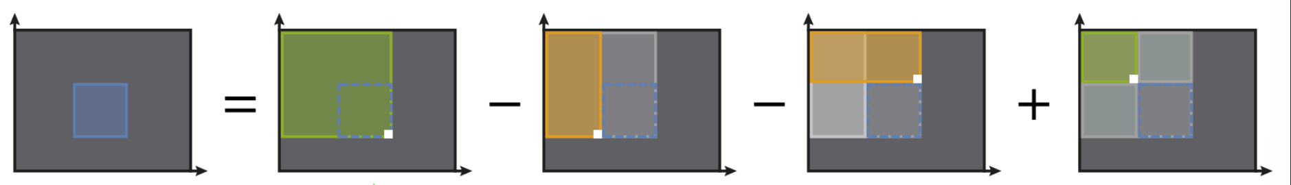
Summed-Area Table (SAT) for Range Query

Essentially doing prefix sum.

• In $(x,y)$$(x, y)$, store the sum of all elements contained inside the rectangle $(0,0)\to (x,y)$$(0,0) \to (x, y)$

• $O(mn)$$O(mn)$ time and storage to build, where $m,n$$m, n$ are width and height, respectively

  • But how to build SAT faster?

[Gamboa et al.]

IV. Moment Shadow Mapping

Motivation

• Approximations fail when scene violates the assumption.

  

  • Overly dark: May be acceptable

  • Overly bright: Light leaking/bleeding (industrial term)

Goal of Moment Shadow Mapping:

• Represent the distribution more accurately

  • But still not too costly to store

• Use higher order moments to represent a distribution

Moments

Partial Reference: [John A. Rice - Mathematical Statistics and Data Analysis 3ed (Duxbury Advanced) (2006, Duxbury Press)]

Definition: The $r$$r$-th moment of a random variable is $E(X^r)$$E(X^r)$, i.e. the expectation of random variable $X$$X$ to $r$$r$.

• VSSM is essentially using the first two orders of moments

What can moments do?

Approximating a distribution more accurately.

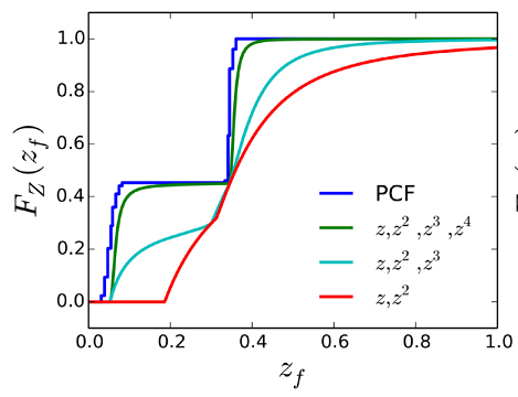
[Peters et al., Moment Shadow Mapping]

• Conclusion: first $m$$m$ orders of moments can represent a function with $m/2$$m/2$ steps

  • Usually, $4$$4$ is good enough to approximate the actual CDF of depth distribution.

• We may restore a CDF given the moment-generating function:

  • The moment-generating function (MGF) of a random variable $X$$X$ is $M(t)=E(e^{tX})$$M(t) = E(e^{tX})$ if the expectation is defined.

  • Properties of MGF:

    • If the moment-generating function exists for $t$$t$ in an open interval containing zero, it uniquely determines the probability distribution.

      The proof depends on Laplace transform. If two random variables have the same MGF in an open interval containing zero, then they have the same distribution.

Moment Shadow Mapping

• Extremely similar to VSSM

• When generating the shadow map, record $z$$z$, $z^2$$z^2$, $z^3$$z^3$, $z^4$$z^4$

  • Packing: Store two 32-bit floating-point into a single one by sacrificing precision.

• Restore the CDF during blocker search & PCF.

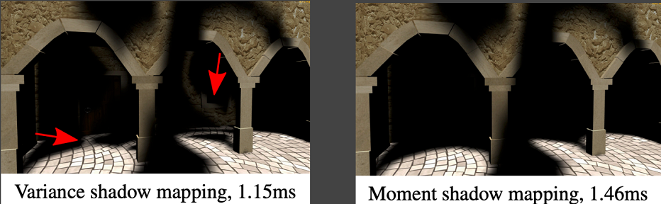
Pros

• Very nice results

Cons

• Costly storage (might be fine)

• Costly performance (during construction)