GAMES202 Lecture 03 - Real-Time Shadows 1
GAMES202_Lecture_03 (ucsb.edu)
I. Shadow Mapping
Reference: Real-Time Rendering, 4th Edition
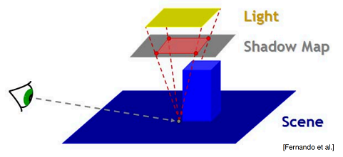
The idea of shadow mapping is to render the scene, using the
To use the shadow mapping, the scene is rendered a second time (Pass 2), but this time with respect to the viewer. As each drawing primitive is rendered, its location at each pixel is compared to the shadow mapping. If a rendered point is farther away from the light source than the corresponding value in the shadow mapping, that point is in shadow. Otherwise, it is not.
Recap
Shadow Mapping is:
A 2-Pass Algorithm
The light pass generates the shadow mapping, or SM
The camera pass uses the SM
Check if each fragment can be illuminated by the light source (using the shadow map)
An Image-Space Algorithm
Pro: No required knowledge of scene's geometry
Con: Causing self-occlusion and aliasing issues
A well-known shadow rendering technique
Basic shadowing technique even for early offline renderings, e.g., Toy Story
| Pass 1 | Pass 2A | Pass 2B |
|---|---|---|
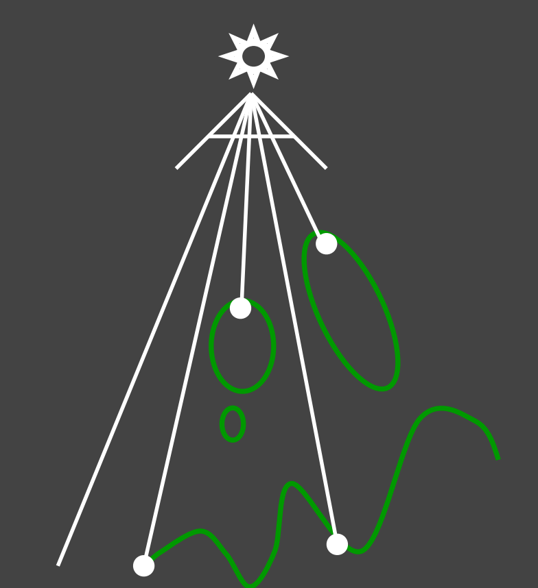 |  |  |
Pass 1
Output a "depth texture" from the light source
For each fragment on that depth texture, record the minimum depth seen from the light source
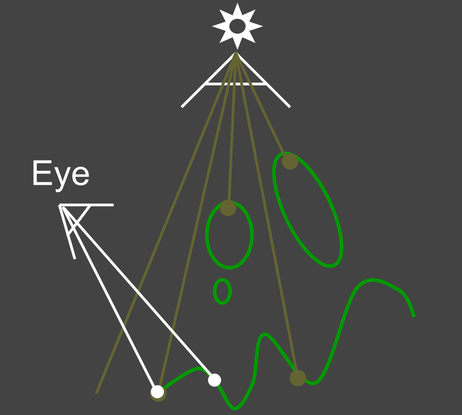
Pass 2
Pass 2A: Render a standard image from the eye
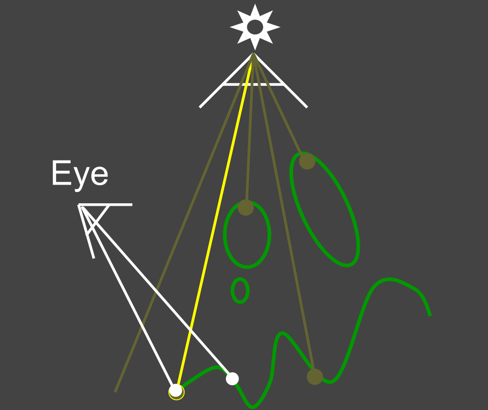
Pass 2B: Project visible points in eye view back to light source. Test the depth.
If the depth does not match the previous one, then the point being rendered is blocked from the light source.
| Depth View | Eye's View (Depth) |
|---|---|
 | 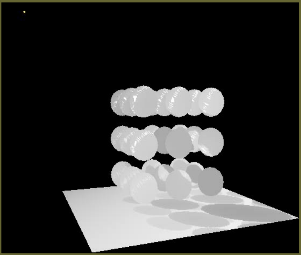 |
Depth View - Viewed from light source
In this figure: the darker the fragment is, the closer the corresponding point on that object is to the light source
Eye's View - Viewed from camera, projecting the depth map onto the eye's view.
Notice how specular highlights never appear in shadows
Notice how curved surfaces cast shadows on each other
Cautions
The definitions of
If you are to use the actual distance, then use that distance at both 2 passes.
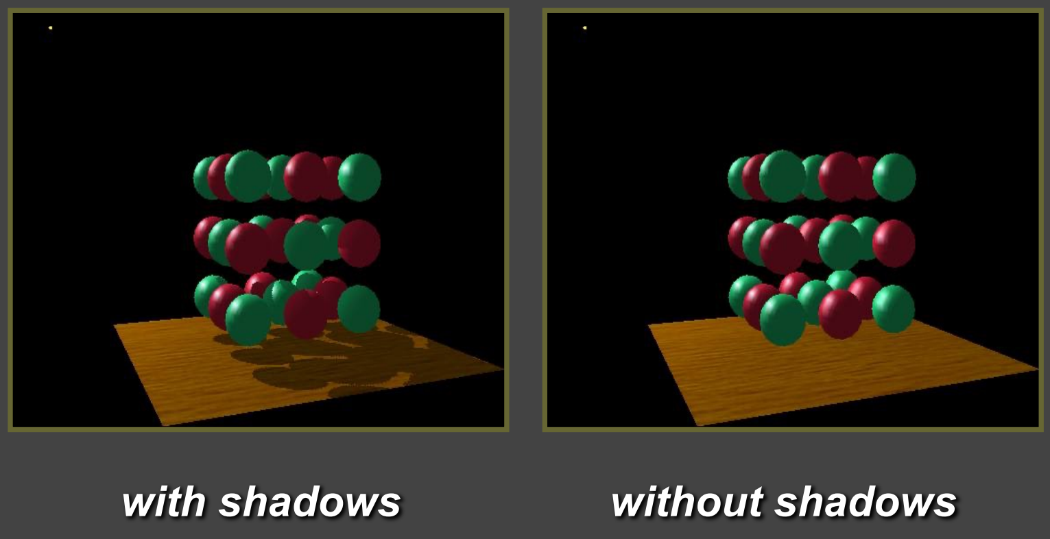
Common Issues and Solutions
Self Occlusion
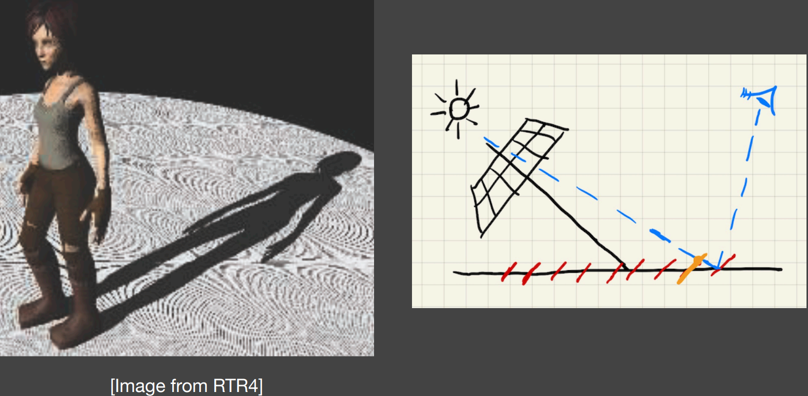
Resolution and floating-point precision count. Notice the red slashes on the right figure.
Each pixel covers an area of the surface, in which the depth is constant (because it is within a single fragment).
The actual depth differs from that recorded in the shadow mapping
The effect is most severe at grazing angle.
The effect is mitigated when the plane used for shadow mapping is parallel to the surface being illuminated.
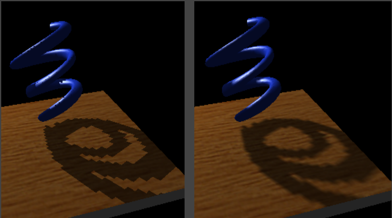
The bias is too low, so self-shadowing occurs. Notice the weird pattern on the ground - they are produced because triangles (that are used to model the ground) shadow themselves.
Adding a (variable) bias to reduce self occlusion
Now the shadow occurs only if the difference exceeds certain threshold:
May be related to viewing angle. If perpendicular to the surface, then little bias. Else, high bias.
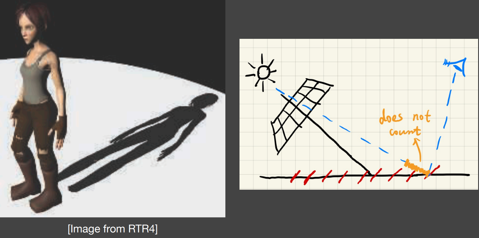
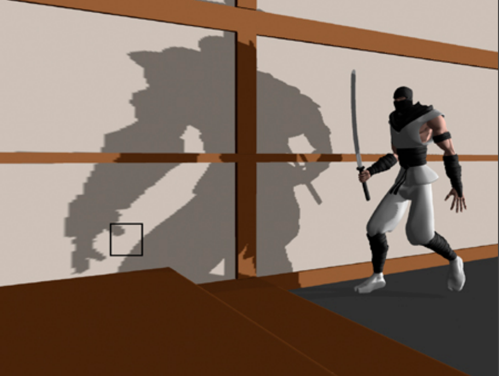
Bias is too high: Introducing detached shadow.
Small object causes the difference between depths to be lied within the bias interval.
Notice the detached shadow on Laura's shoes.
Second-Depth Shadow Mapping
Store the second-minimum depth when generating the shadow map.
Using the midpoint between first and second depths in the SM.
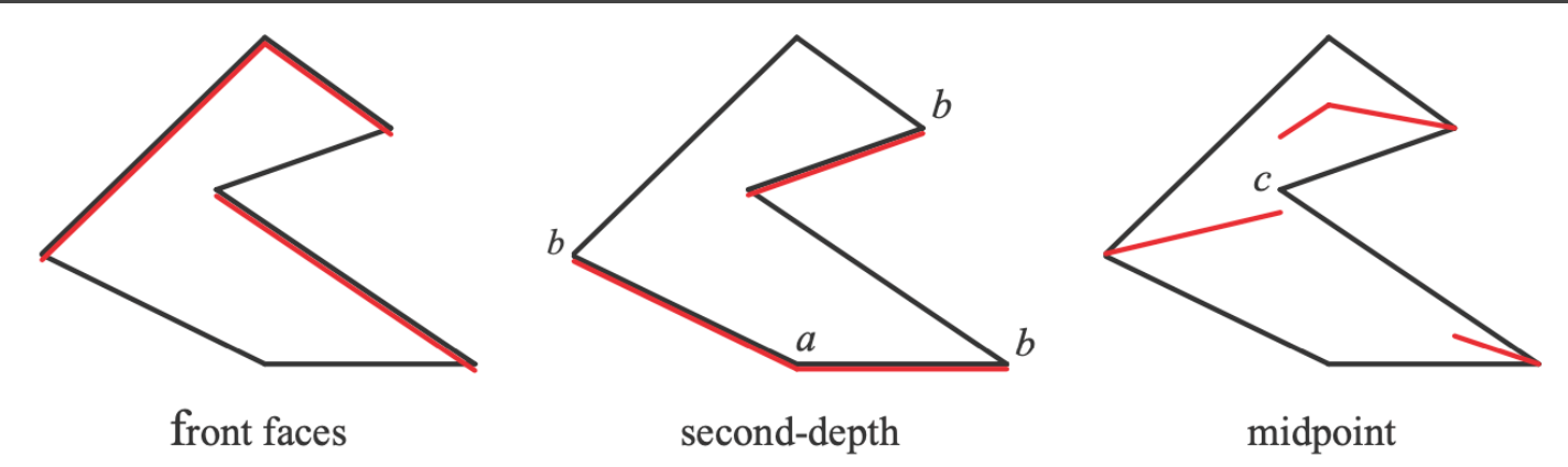
Assume the light source is directly above.
Requires objects to be watertight:
Cannot describe planes without volume. (Can be solved with some tricks)
The overhead may not worth it:
RTR does not trust in complexity: The actual time may be doubled or tripled or even more.
Aliasing
The resolution still counts: The area covered by a single fragment inside the shadow maps has a constant depth. Solution: change the resolution of shadow maps:
Shadow Maps with Dynamic Resolution
Cascaded Shadow Maps
Convolutional Shadow Maps
II. The Math behind Shadow Mapping
Approximating the Rendering Equation
In real-time rendering, we care about fast and accurate approximation. (Approximately equal)
An important approximation throughout RTR:
Approximate the result of integration by averaging
When is it (more) accurate?
When the support of
The support of a real-valued function
When
When
The rendering equation with term
can be approximated as, if not considering term regarding to self-emittance,
Separate visibility from the integration. The right part now remains only the direct shading.
This is the basic concept behind shadow mapping.
When is it accurate?
Small support: Point/directional lighting
Smooth integrand: Diffuse BSDF/Constant radiance area lighting.
Will be reviewed again when discussing Ambient Occlusions.
III. Percentage Closer Filtering (PCF) and Percentage Closer Soft Shadows (PCSS)
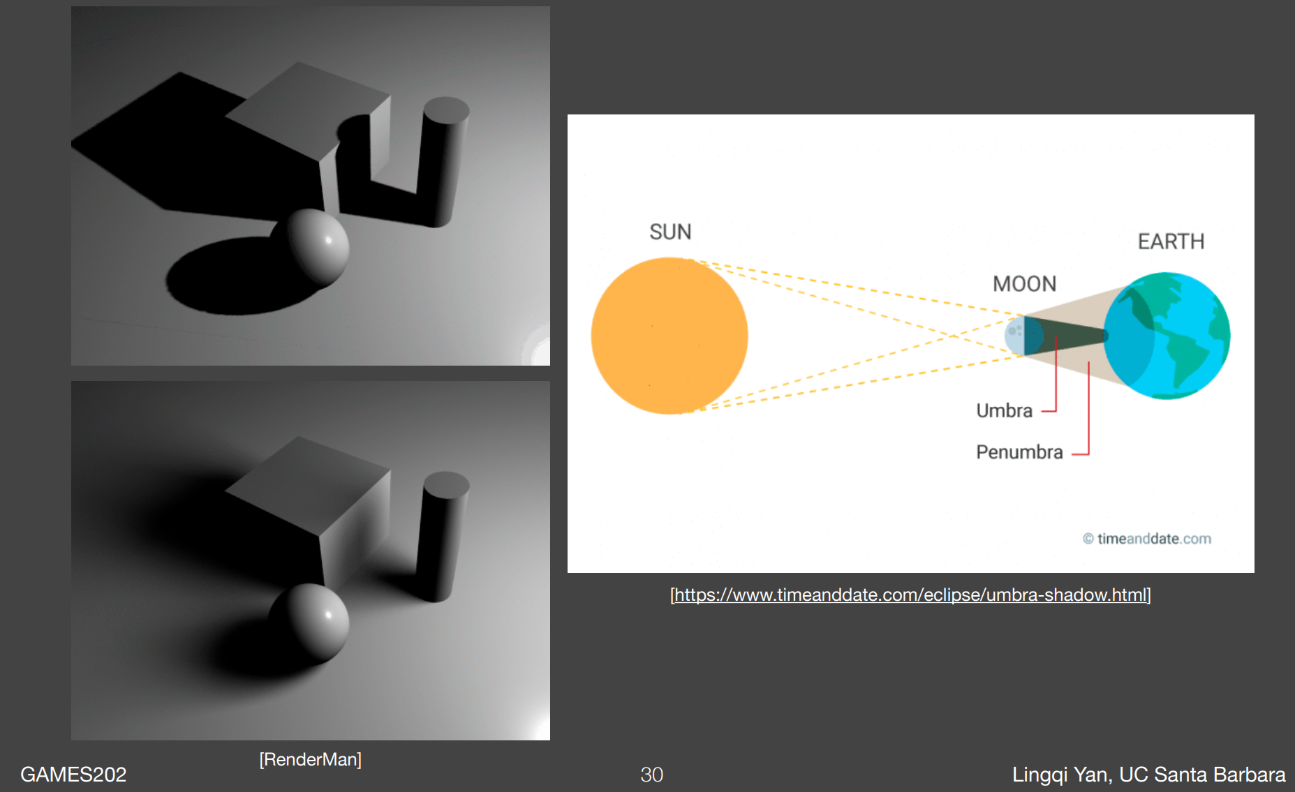
Upper: Point Light, umbra only
Inside the umbra of a light source, the viewer cannot see that light source.
Lower: Area Light, with penumbra
Inside the penumbra of a light source, the viewer can see only part of that light source.
Percentage Closer Filtering
Provides anti-aliasing at shadows' edges
Not for soft shadows (PCSS, which is for soft shadows, will be introduced later)
Filtering the results of shadow comparisons
Averaging the results of shadow comparisons
Why not filter the shadow map?
Texture filtering just averages color components:
You'll get blurred shadow map first
Averaging depth values and comparing then will still lead to a binary visibility.
The Algorithm
Compute the visibility term in the rendering equation:
Instead of performing a single query, perform multiple (e.g.,
Method: In the shadow map (figure below), query the neighboring region of point
Querying the fragment: the farther the fragment is to the light source, the blurrier its corresponding shadow will be.
Then, averages the results of comparisons.
For example:
For point
Compare its depth
Get the compared results, e.g.,
Take the average to get visibility, e.g.,
Wrong example: filtering on the result
Problems
Does filtering size matter?
Smaller -> Sharper
Larger -> Softer
Can we use PCF to achieve soft shadow effects?
Using a larger filter size leads to visual approximation of soft shadows
Key thoughts:
From hard shadows to soft shadows
What's the correct size to filter?
Is the produced shadow uniform?
No. The closer the object is to the projecting surface, the sharper the projected shadow will be.
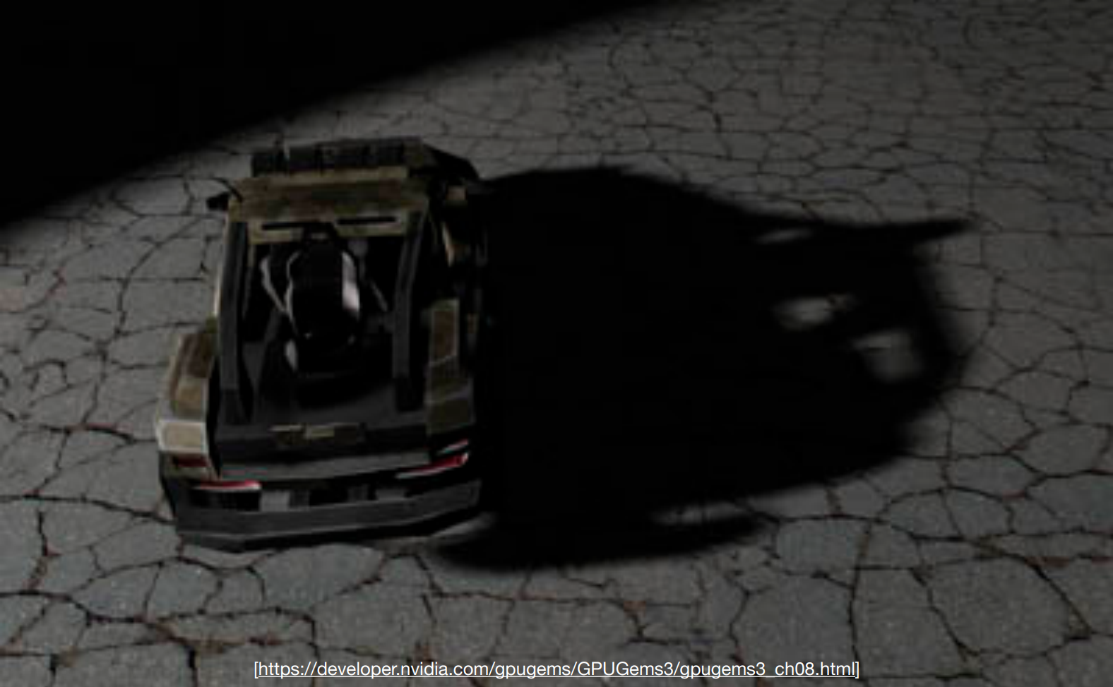
Percentage Closer Soft Shadows

The shadow becomes sharper as the tip gets closer to the plane. Softer in the other direction.
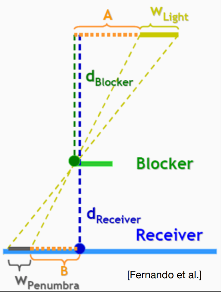
Blocker distance: Averaged projected blocker depth.
Average samples of depth in an area
Projected so as to get the perpendicular distance
Shadow map cannot be produced with an area light.
The soft shadow created by the area light, is simulated by:
First using a point light to generate the shadow map,
Then specify the dimension of that light when doing calculation, i.e. post-processing
The ratio in the formula corresponds to word percentage in its name
PCSS - The Complete Algorithm
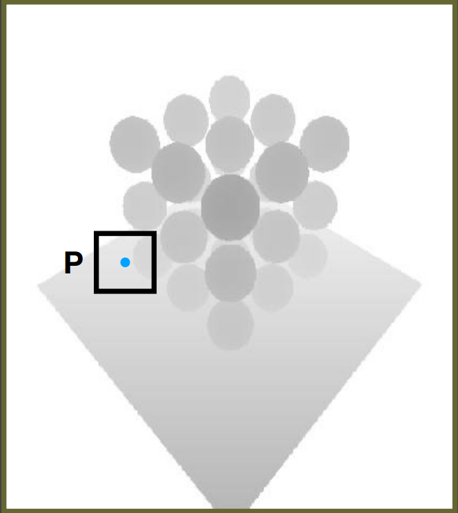
Blocker Search:
Get the average blocker depth in a certain region inside the shadow map:
In a region, what is the average depth of the area that covers the shading point?
Penumbra Estimation:
Use the average blocker depth to determine filter size
Percentage Closer Filtering
Problems
Which region to perform blocker search? What size?
Can be set constant (e.g.,
Depends on the size of light, and distance between receiver and the light:
When estimating the blocker depth, create a cone as the figure shows, and use the projected area on the shadow map covered by the cone.
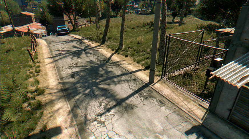
Video Game: Dying Light