GAMES101 Lecture 22 - Animation Cont.

GAMES101_Lecture_22.pdf

Outline

• Single Particle Simulation

  • Explicit Euler Method

  • Instability and Improvements

• Rigid Body Simulation

• Fluid Simulation

I. Single Particle Simulation

For similicity we may write vectors in the same way as scalars.

Vector Field and Ordinary Differential Equation (ODE)

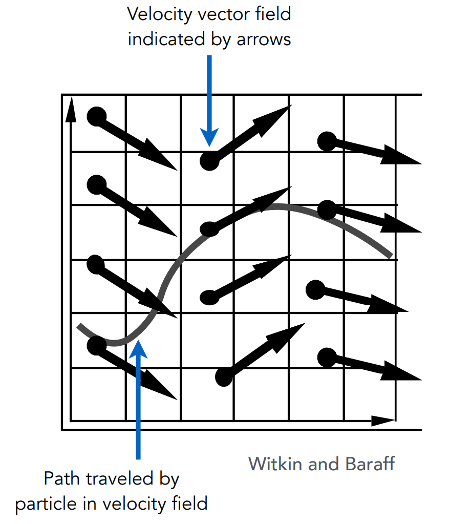
Assume the motion of a particle is determined by a velocity vector field that is a function of position and time:

Computing the position of that particle over time requires solving a first-order ordinary differential equation (ODE):

Solve the ODE subject to a given initial particle position $x_0$$x_0$ by using forward numerical integration.

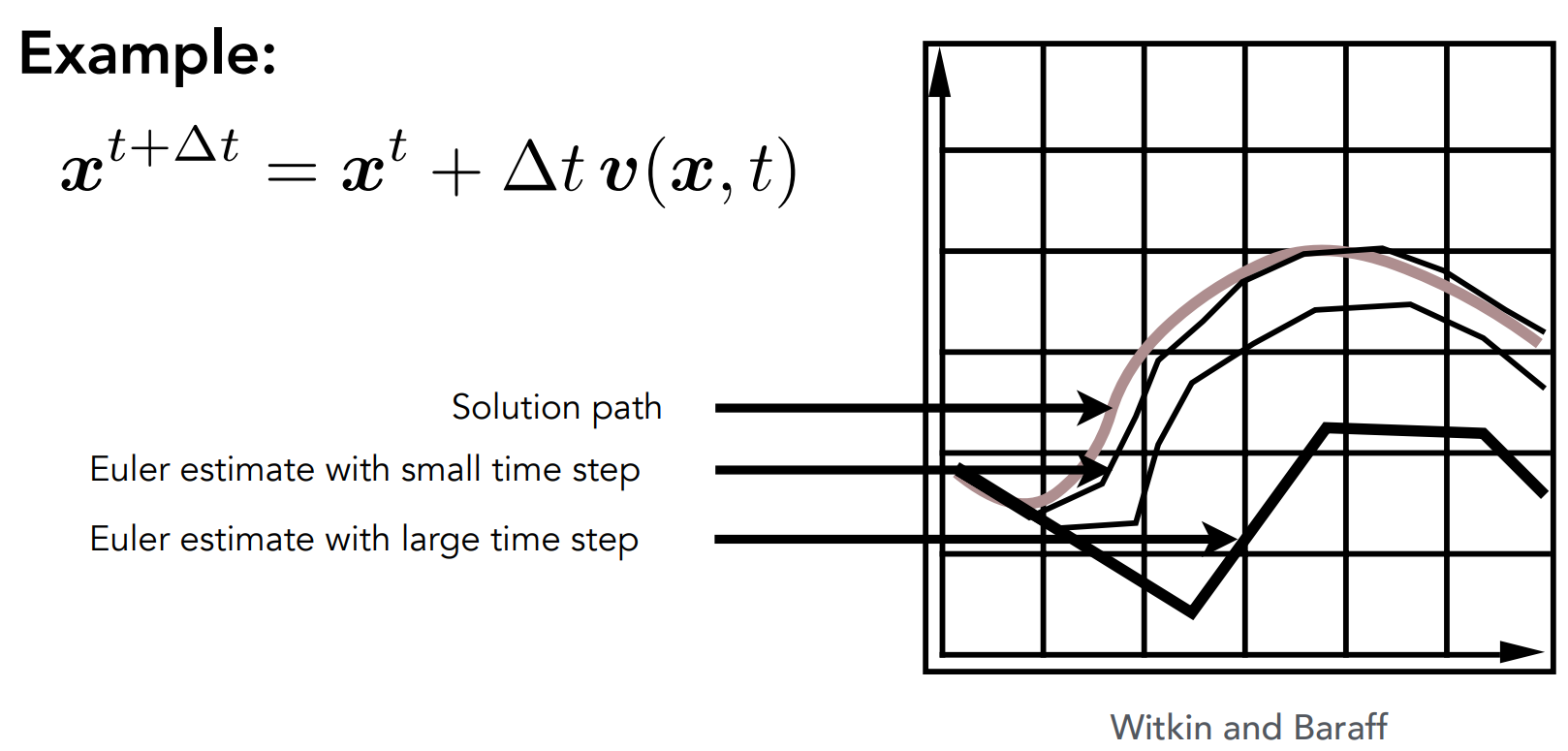
Euler's Method

Euler's Method, a.k.a. Forward Euler, Explicit Euler, is

• a simple iterative method,

• commonly used,

• very inaccurate, and

• most often goes unstable.

The rightside of the equation consists of only values at present.

Errors

Errors accmulate as the integration goes, and euler integration is particularly bad.

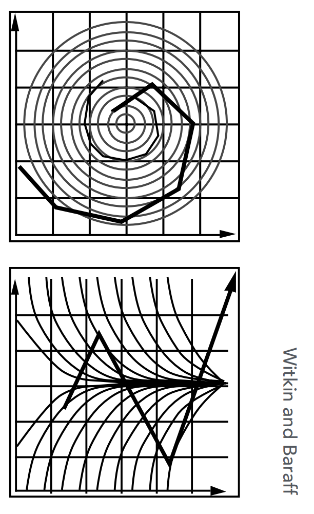
Instability

• Inaccuracy increases as step $\mathrm{\Delta }t$$\Delta t$ increases

• Instability is a common, serious problem that can cause simulaton to diverge.

Resolving Errors and Instability

Solving by numerical integration with finite differences leads to two problems:

• Errors:

  • Errors at each time step accmulate. Accuracy descrease as simualtion proceeds.

  • Accuracy may not be critical in graphics applications.

• Instability:

  • Errors can compound, causing the simualtion to diverge even when the underlying system does not.

  • Lack of stability is a fundamental problem in simulation, and cannot be ignored.

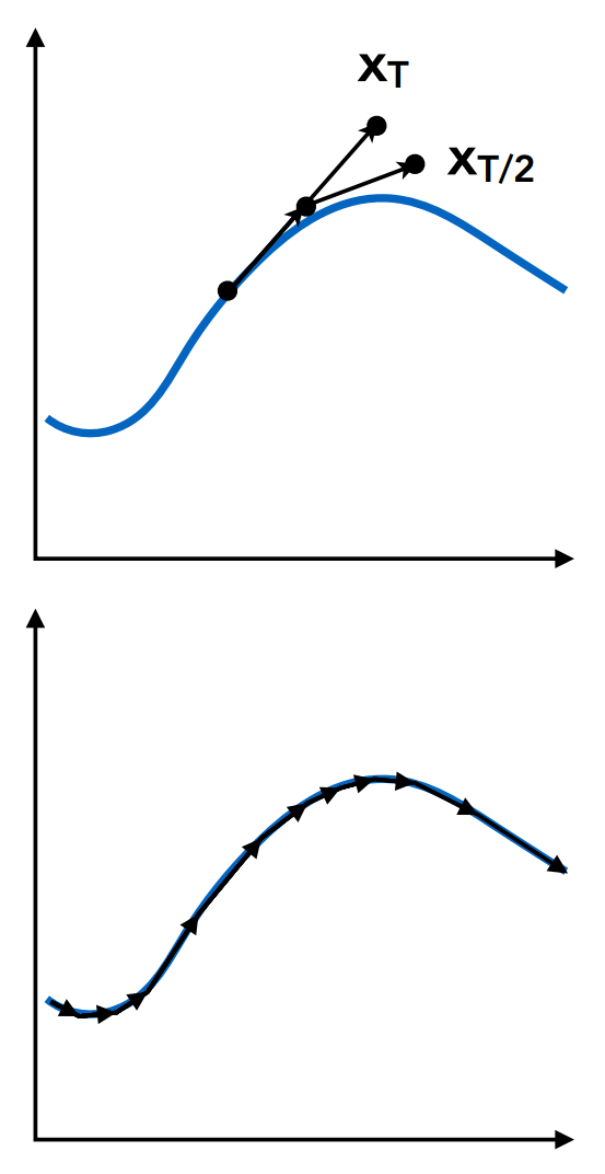
• Midpoint Method/Modified Euler

  • Average velocities at start and endpoint.

• Adaptive Step Size

  • Compare one step and two half-steps recursively until the error is acceptable.

• Implicit Methods

  • Use the velocity at the next time step (hard)

• Position-Based/Verlet Integration

  • Constraint positions and velocities of particles after step $\mathrm{\Delta }t$$\Delta t$

Midpoint Method/Modified Euler

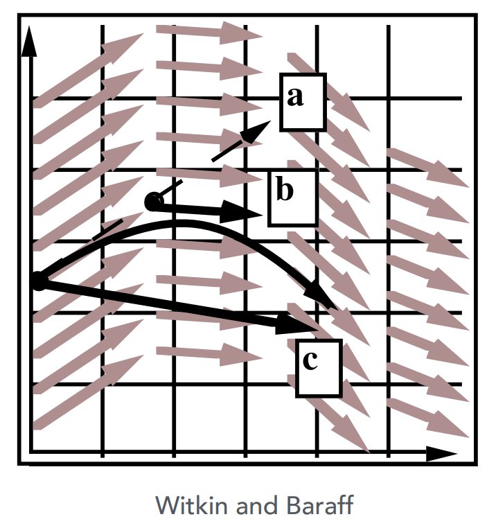
1. Compute Euler step $(a)$$(a)$

2. Compute derivative at the midpoint of Euler step $(b)$$(b)$

3. Update position using midpoint derivative $(c)$$(c)$

• Averaging velocity at start and end of step gets better results. (Applying second derivatives)

Adaptive Step Size

• Technique for choosing step size based on error estimation

• Practical

• May need very small steps

Repeat until error is below threshold:

1. Compute $x_T$$x_T$ an Euler step, size $T$$T$

2. Compute $x_{T/2}$$x_{T/2}$ two Euler steps, size $T/2$$T/2$

3. Compute error $ϵ=\Vert x_T-x_{T/2}\Vert$$\epsilon = \norm{x_T - x_{T / 2}}$

4. If $ϵ>C$$\epsilon > C$, a predefined threshold, then reduce step size $T$$T$ and try again.

Implicit Euler Method

• Informally called Backward Methods.

• Use derviatives in the future for the current step

• Solve nonlinear problem for $x_{t+\mathrm{\Delta }t}$$x_{t + \Delta t}$ and ${\dot{x}}_{t+\mathrm{\Delta }t}$$\dot{x}_{t + \Delta t}$

  • However, we likely do not know ${\ddot{x}}_{t+\mathrm{\Delta }t}$$\ddot{x}_{t + \Delta t}$ if the position is unknown

  • And we need to compute a numerical solution

• Use root-finding algorithm, e.g. Newton's method

• Much better stability:

  • Measured by local truncation error (for each step) and total accumulated error (overall)

  • Order of error w.r.t. step matters more than the absolute value

  • Implicit Euler has order 1, which means that

    • Local truncation error: $O(h^2)$$O(h^2)$, and

    • Global trucnation error: $O(h)$$O(h)$, where $h$$h$ corresponds to the size of step

  • $O(h)$$O(h)$ - halving $h$$h$ leads to halving the error.

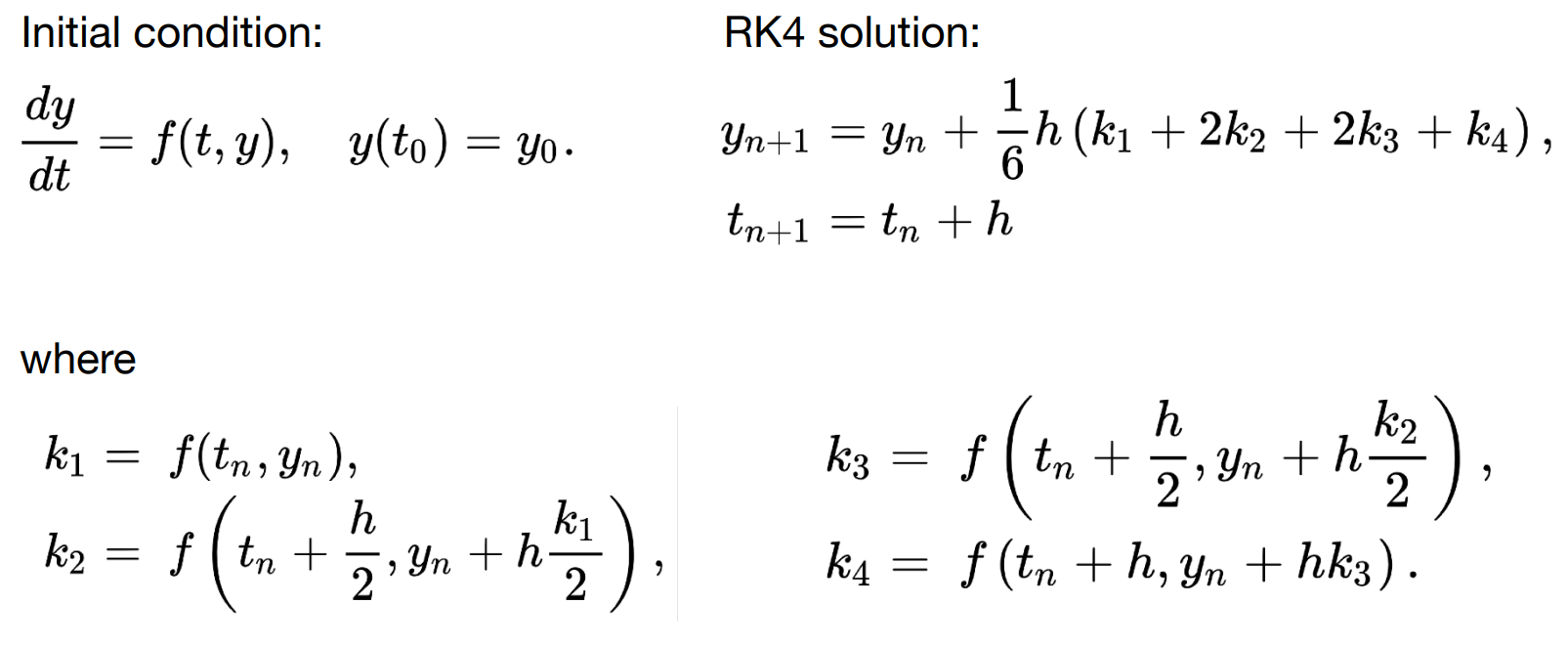
Runge-Kutta Families

A family of advanced methods for solving ODEs.

• Especially good at dealing with non-linearity

• RK4, or the order-four version, is the most widely used

Position-Based/Verlet Integration

• After modified Euler forward-step, constrain positions of particles to prevent divergent, unstable behavior

• Use constrainted positions to calculate velocity

• Both of these ideas will dissipate energy, stablize

Pros/Cons

• Fast and simple

• Not physically based, violates conservation of energy

II. Rigid Body Simulation

Simple case:

• Since the rigid body has all its components fixed, simulation is similar to that of a particle, but with a bit more properties:

  $$\begin{array}{c}\frac{\mathrm{d}}{\mathrm{d}t}\left[\begin{array}{c}x\\ \theta \\ \dot{x}\\ \omega \end{array}\right]=\left[\begin{array}{c}\dot{x}\\ \omega \\ f/m\\ \tau /I\end{array}\right]\end{array}$$

  where

  • $x$$x$ is the position,

  • $\theta$$\theta$ is the angle of rotation,

  • $\omega$$\omega$ is the angular velocity,

  • $f$$f$ is the forces,

  • $\tau$$\tau$ is the torque, and

  • $I$$I$ is the moment of inertia.

III. Fluid Simulation

A Simple Position-Based Method

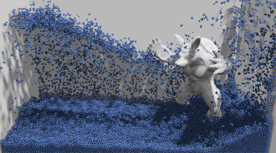
Key idea:

• Assumptions:

  • Water is composed of small rigid-body spheres

  • Water cannot be compressed

    • As long as the density changes somewhere, it should be corrected via changing the position of particles

• Need to know the gradient of the density anywhere w.r.t each particle's position

• Do gradient descent.

Eulerian vs. Lagrangian

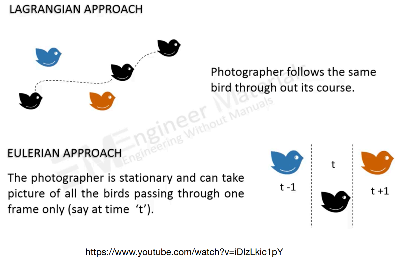
• Lagrangian: explictly compute the position of each particles

• Eulerian: Separate the space into a grid, compute the change happened inside the grid

Material Point Method (MPM)

Hybrid, combining Eulerian and Lagrangian views:

• Lagrangian: consider particles carrying material properties

• Eulerian: use a grid to do numerical integration

• Interaction: particles transfer properties to the grid, grid performs update, then interpolate back to particles