GAMES101 Lecture 17 - Materials and Appearances
I. Materials and Appearances

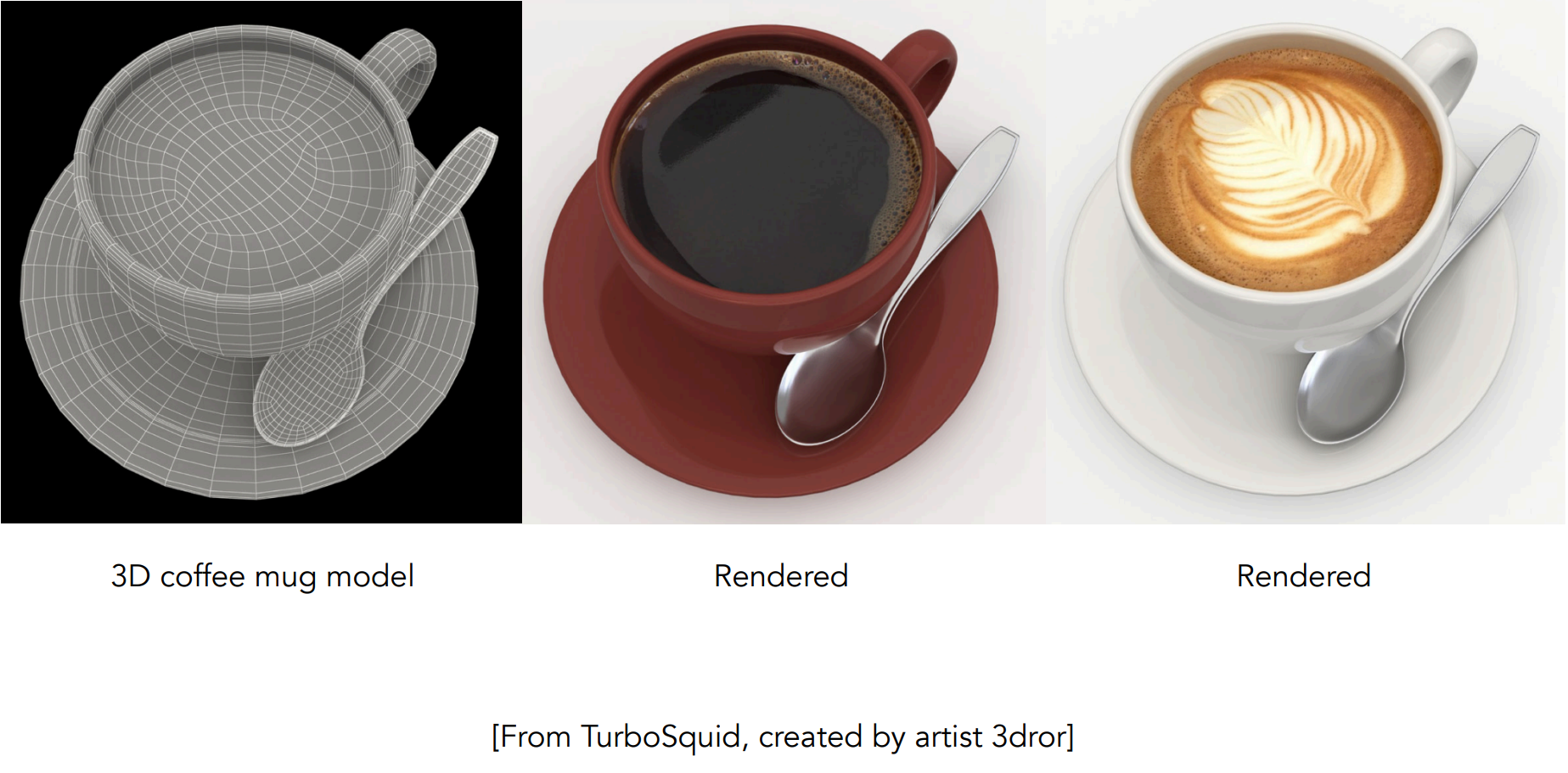
Textures and appearances are closely related:
Under different lighting conditions textures appears to be different.
Some of the features from natural materials:
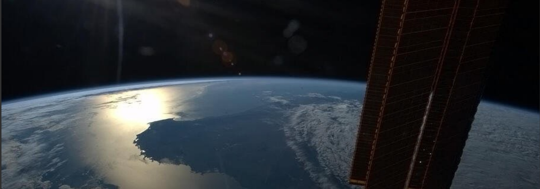
Water
Scattering
Hair/Fur
Clothes
Subsurface Scattering (SSS)
...
The term material is equivalent to BSDF.
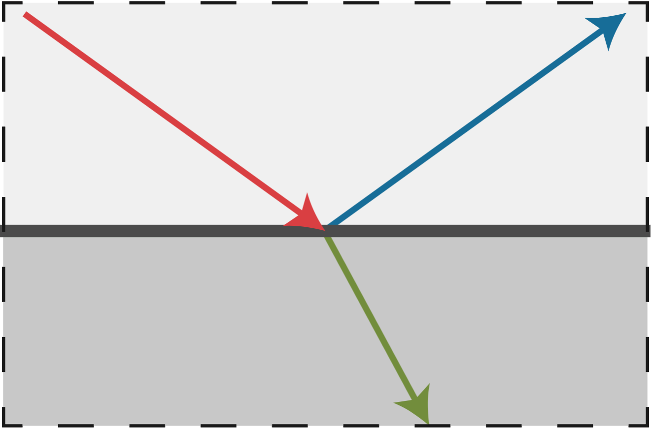
Bidirectional Scattering Distribution Function, BSDF
The generalization of BRDF and BTDF (Bidirectional Transmittance Distribution Function), which takes both refraction and reflection into consideration.
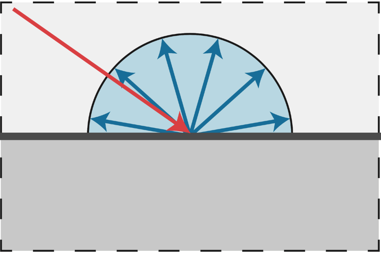
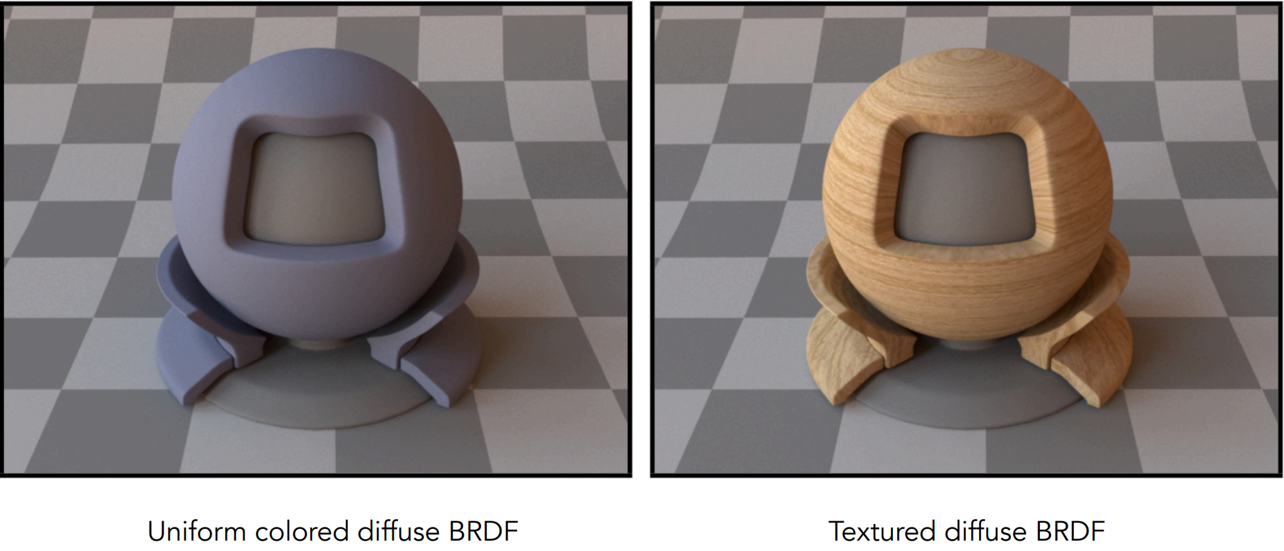
Diffuse/Lambertian Material
From [Mitsuba render, Wenzel Jakob, 2010
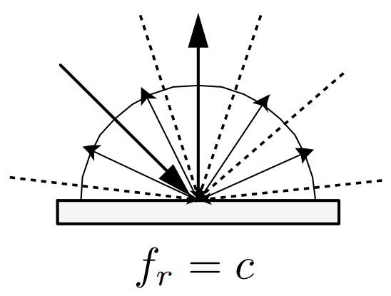
Light is equally reflected in each output direction.
Suppose the incident lighting is uniform in radiance, and without self-emission we have:
If the material absorbs no light, then
On lambertian material we have
in which
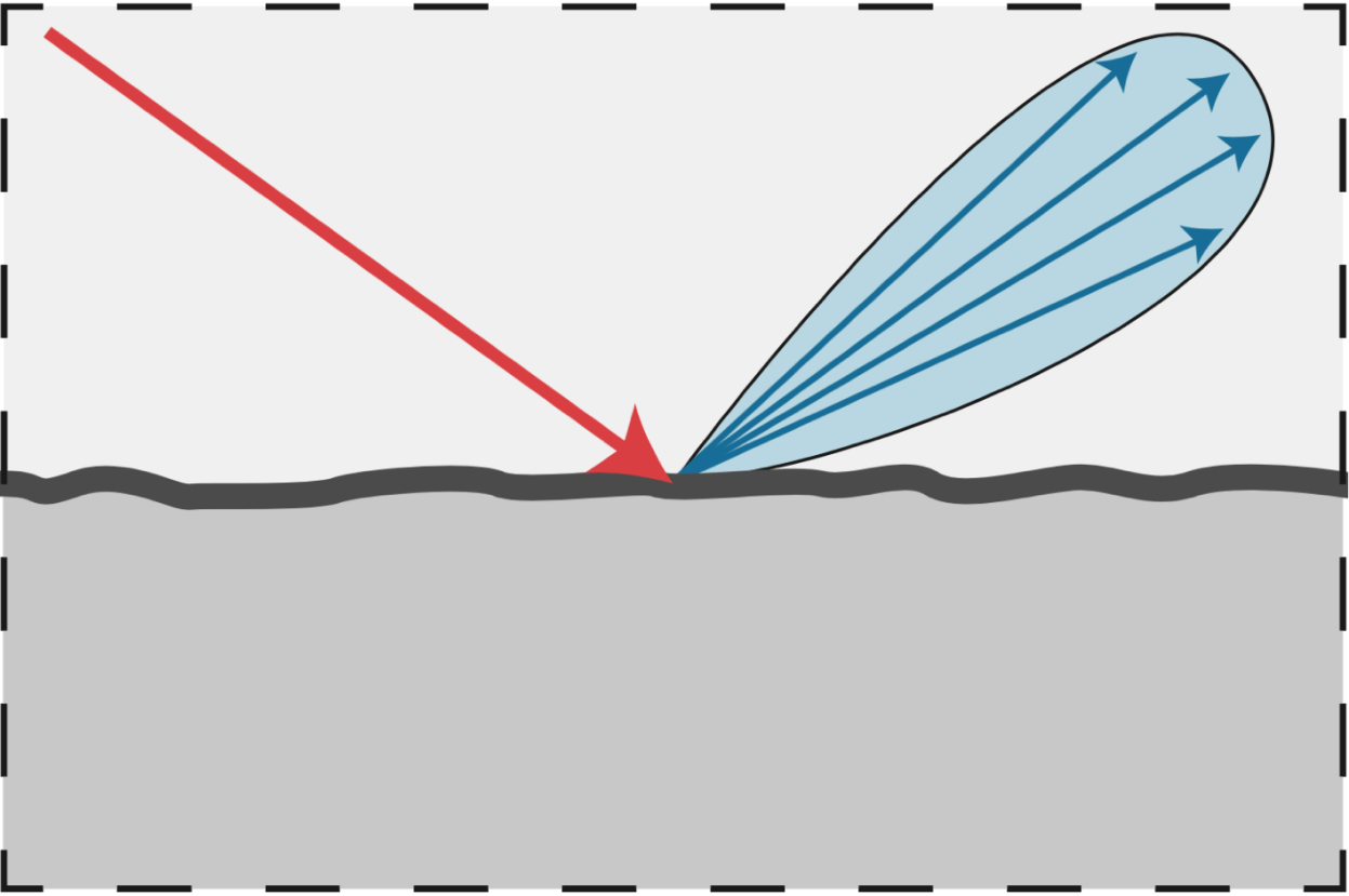
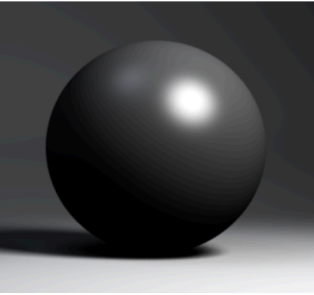
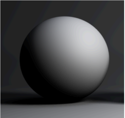
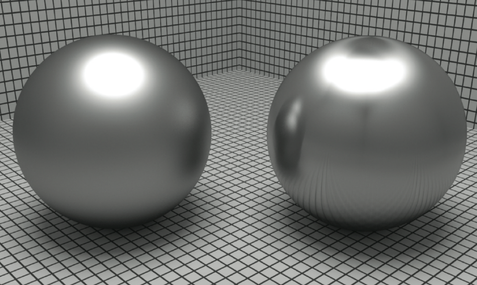
Glossy Material
From [Mitsuba render, Wenzel Jakob, 2010
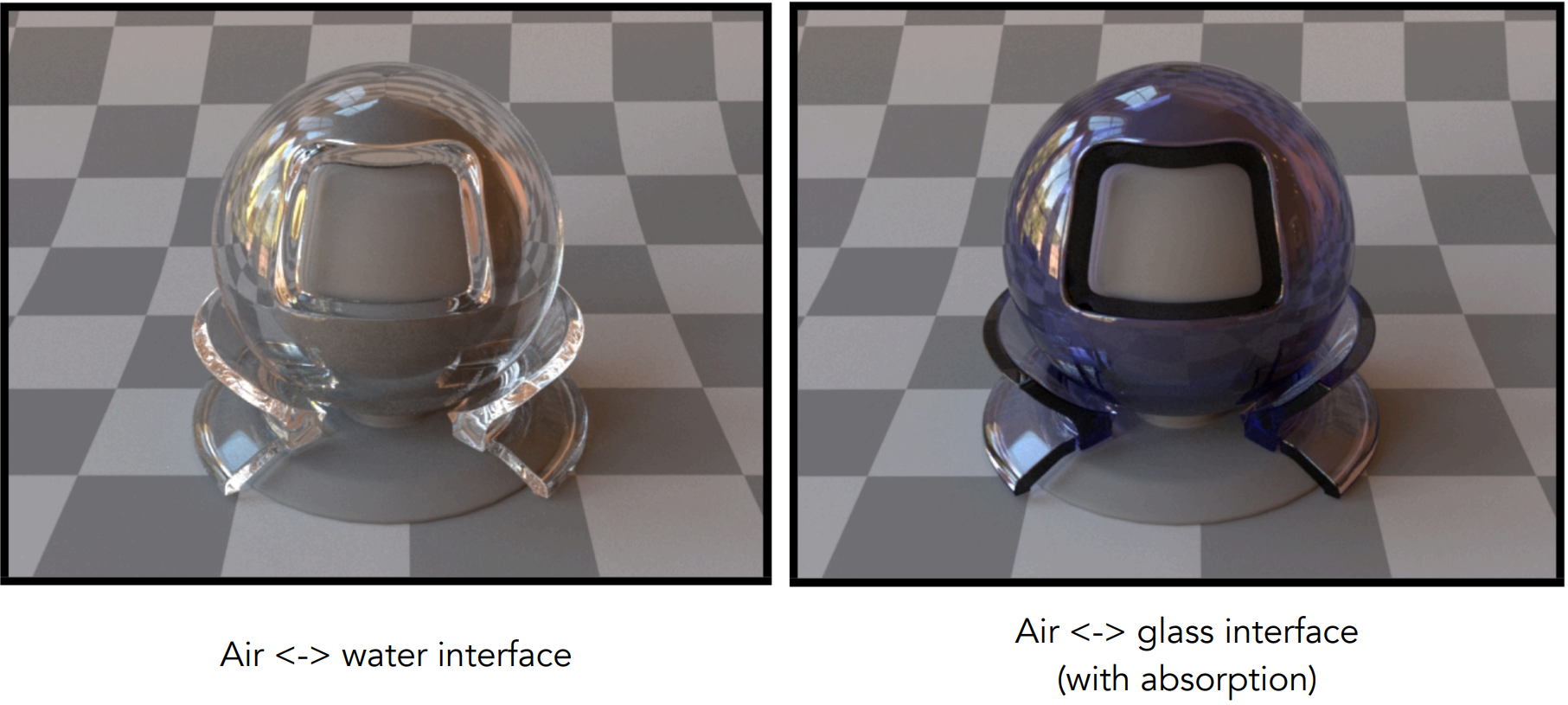
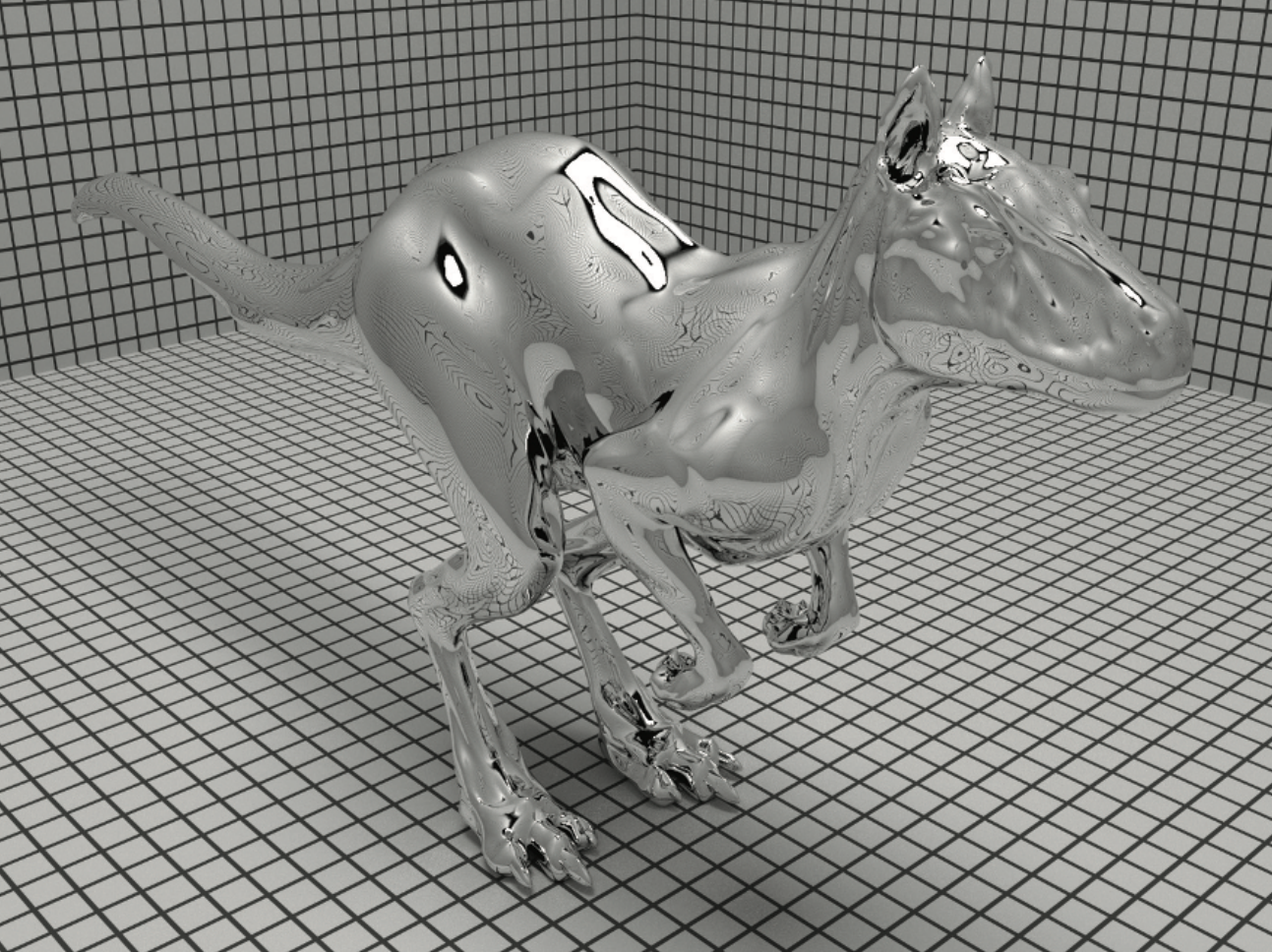
Ideal Reflective/Refractive Material
From [Mitsuba render, Wenzel Jakob, 2010
Part of the spectrum is absorbed by the underlying material.
Perfect Specular Reflection
From PBRT
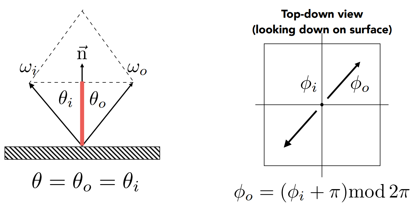
BRDFs for the perfect specular reflection are difficult to write.
Related to the
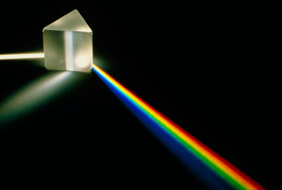
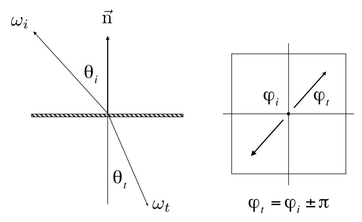
Specular Refraction
Light refracts when it enters a new medium.
Snell's Law
Transmitted angle depends on
index of refraction (IOR) for incident ray
IOR for exiting ray
| Medium | Vaccum | Air (sea level) | Water ( | Glass | Diamond |
|---|---|---|---|---|---|
| 1.0 | 1.00029 | 1.333 | 1.5-1.6 | 2.42 |
Index of frefraction is wavelength dependent. These are averages.
Law of Refraction
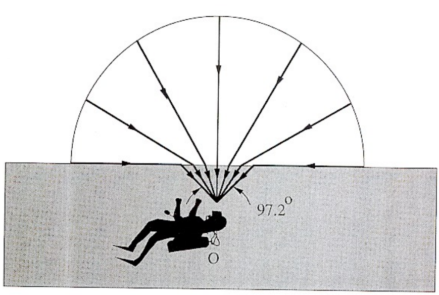
Definition: Total internal reflection: When light is moving from a more optically dense medium to a less optically dense medium, i.e.,
then light incident on boundary from large enough angle will not exit the medium. The critical angle can be computed from equation
Snell's Window/Circle
Fresnel Reflection/Term
Reflectance depends on incident angle (and polarization of light).
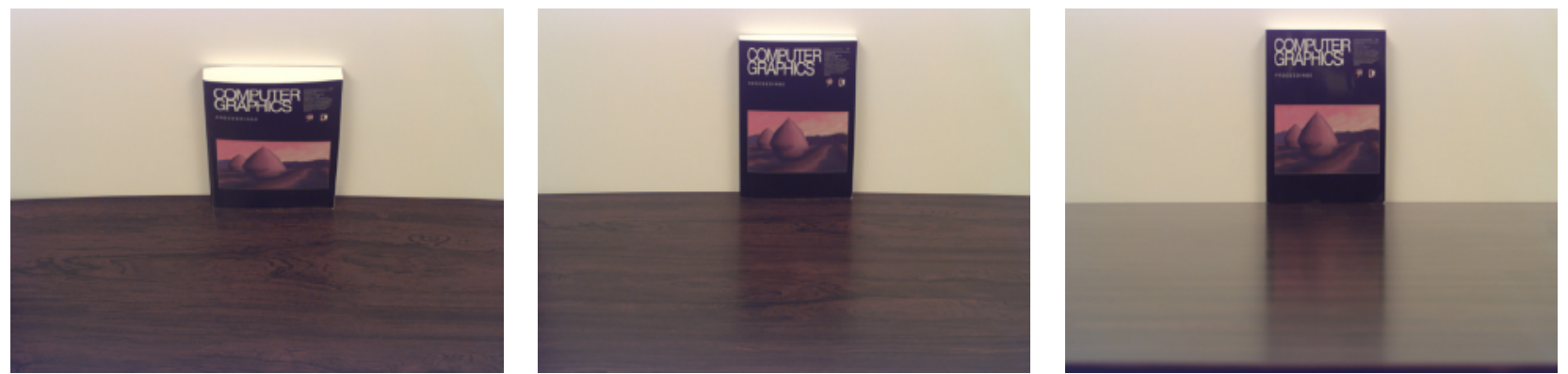
This example: reflectance increases with grazing angle [Lafortune et al. 1997]
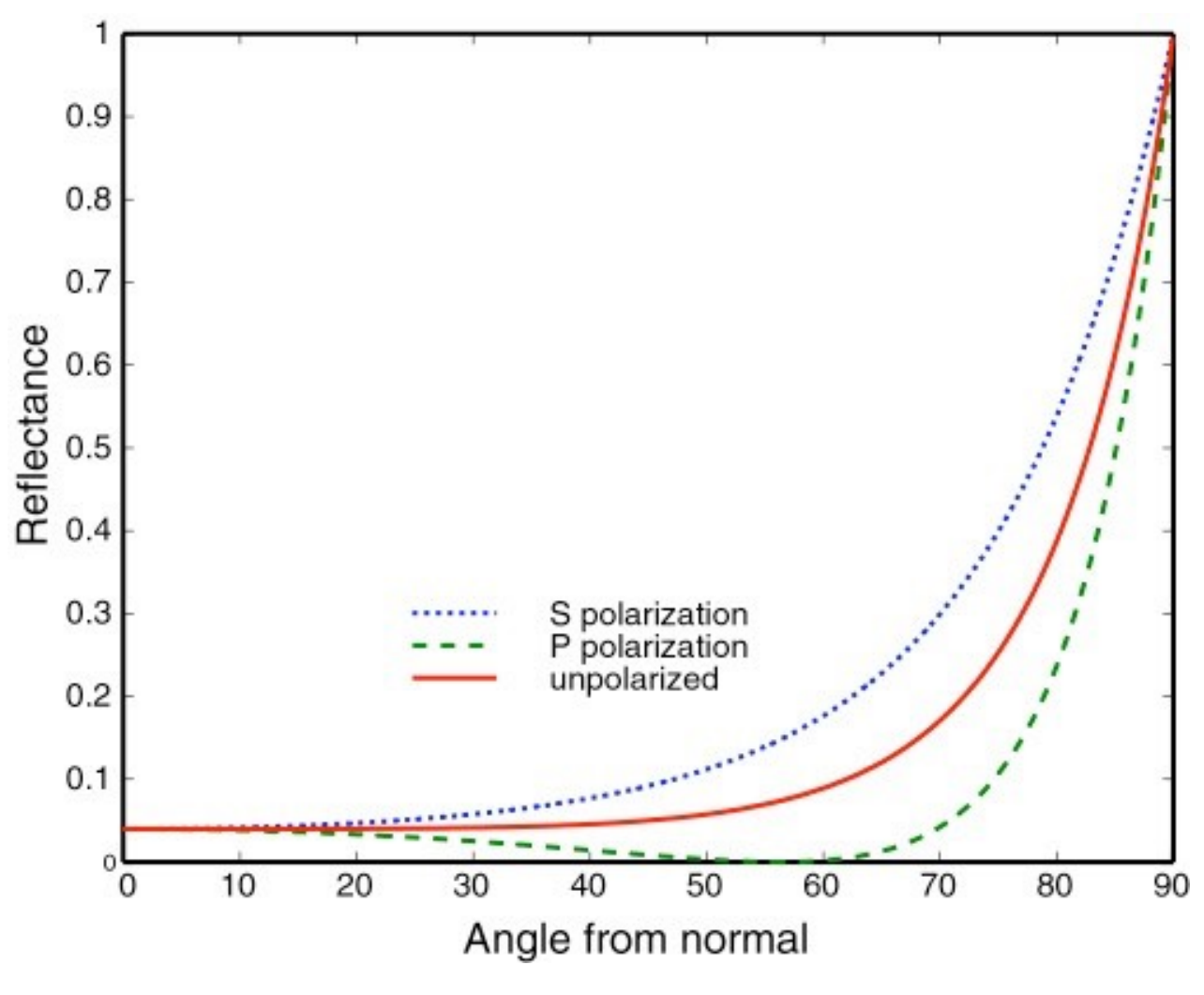
Fresnel Term
Polarization: The component of the electric field parallel to the incidence plane is termed p-like (parallel) and the component perpendicular to this plane is termed s-like (from senkrecht, German for perpendicular). (Wikipedia)
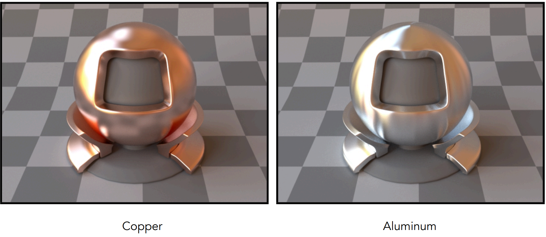
Dielectric,
Conductor:
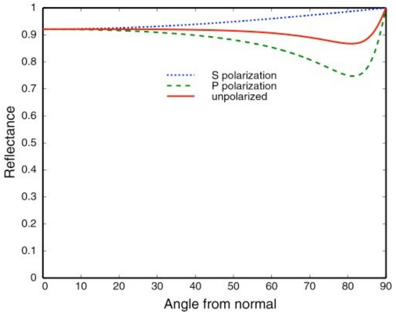
Conductors have negative indices of refraction.
Formulae
Accurate: polarization taken into consideration
Approximate: Schlick's approximation
Microfacet Material
State of art.
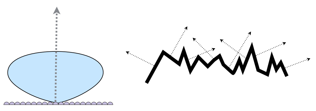
Microfacet Theory
Rough surface:
Macroscale: flat & rough
Microscale: bumpy & specular
Microfacet: individual elements of surface act like mirrors
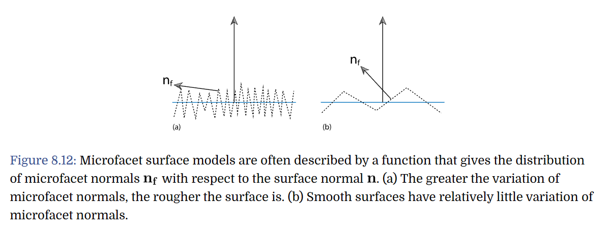
Key: The distribution of their normals. Each microfacet has its own normal.
Concentrated <==> Glossy
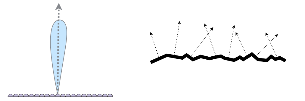
Spread <==> Diffuse
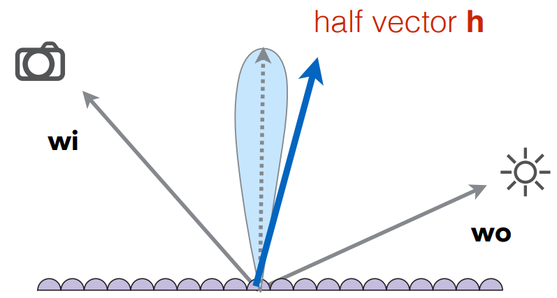
Microfacet BRDF:
In which:
Microfacets may block each other.
Happens often when lights are near the grazing angle.
How many normals are there that match the direction of
Isotropic/Anisotropic Materials (BRDFs)

Key: Directionality of the underlying surface.
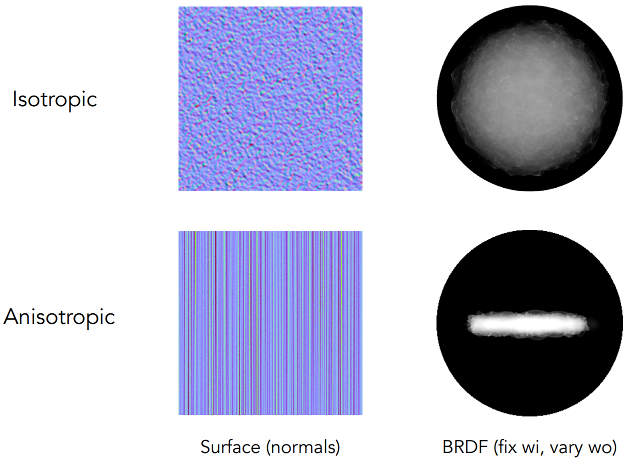
Anisotropic: Reflection depends on azimuthal angle
Results from oriented microstructure of the surface, e.g.
Brushed Metal
Nylon
Velvet
II. Further on BRDFs
Properties of BRDFs
Non-negativity: On any point,
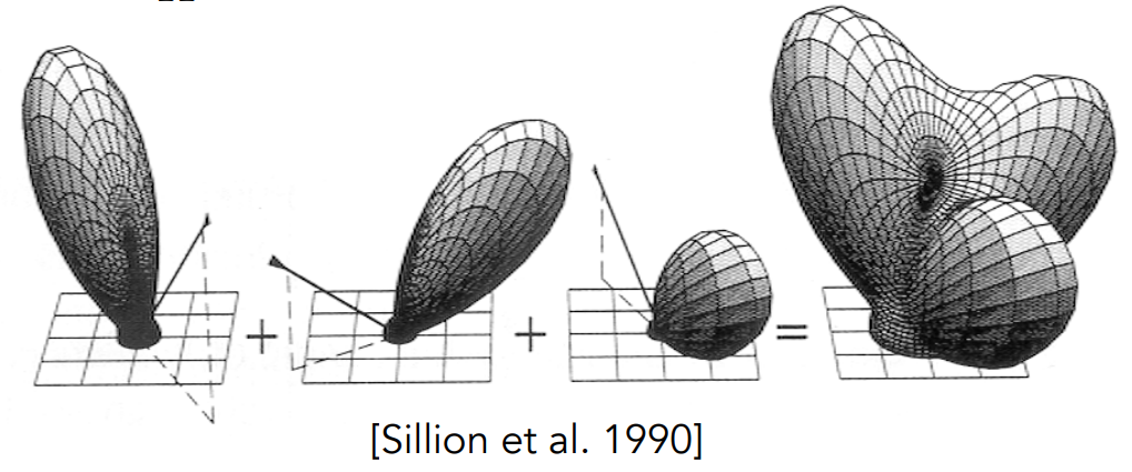
Linearity: BRDFs can be directly summed.
The nature of integration make BRDFs addable.
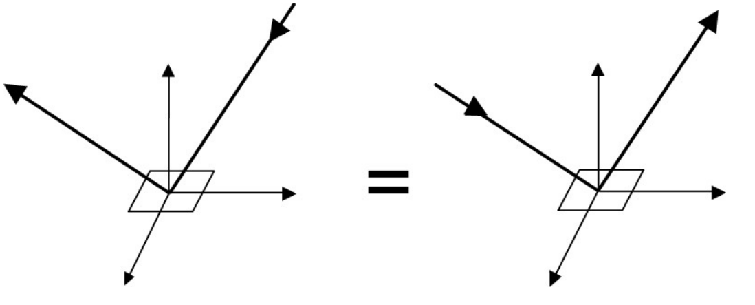
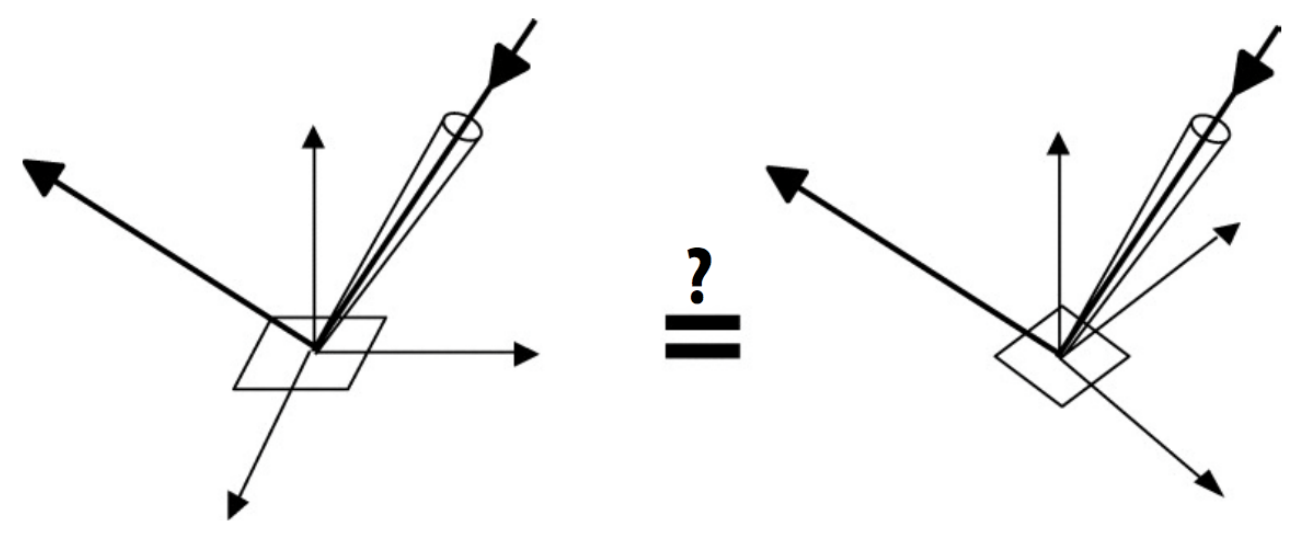
Reciprocity Principle
Energy Conservation
Isotropic/Anisotropic
If isotropic:
Then from reciprocity we have
Measuring BRDFs
Target:
Avoid need to develop/derive models
Automatically includes all of the scattering effects present
Can accurately render with real-world materials
Useful for product design, special effects, ...
General Approach
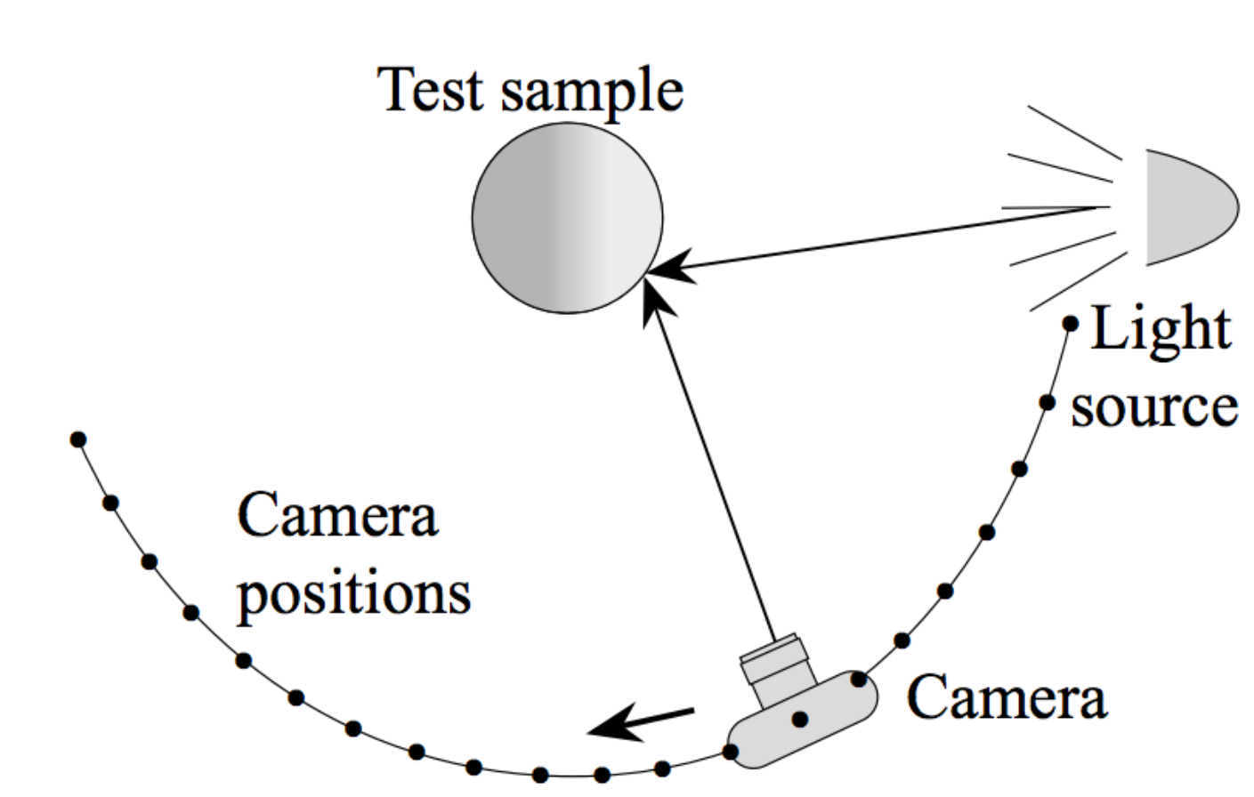
For each outgoing direction
move light to illuminate surface with a thin beam from
For each incoming direction
move sensor to be at direction
measure incident radiance
Gonioreflectometer:
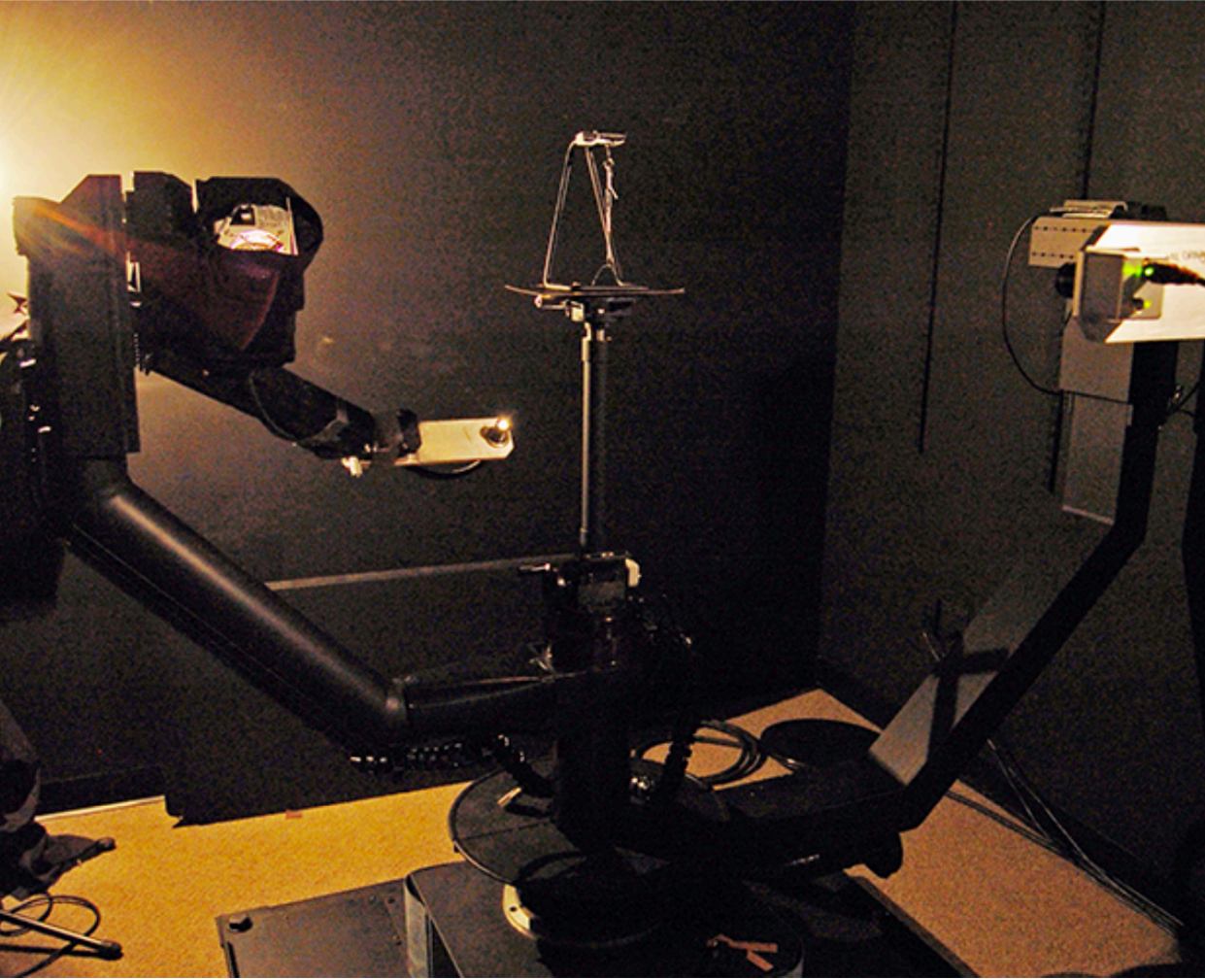
Spherical gantry at UCSD
Improving Efficiency
Isotropic surfaces reduce dimensionality from 4D to 3D
Reciprocity reduces # of measurements by half
Clever optical systems
Challenges
Accurate measurements at grazing angles
Important due to Fresnel effects
Measuring with dens enough sampling to capture high frequency specularities
Retro-reflection
Spatially-varying reflectance
...
Representing Measured BRDFs
Desirable qualities:
Compact representation
Accurate representation of measured data
Efficient evaluation for arbitrary pairs of directions
Good distributions available for importance sampling
Tabular Representation
MERL BRDF Database [Matusik et al. 2004],
Store regularly-spaced samples in
Better: reparameterize angles to better match specularities
Generally need to resample measured values to table
Very high storage requirements
Appendix A: Microfacet Models
Reference: Microfacet Models (pbr-book.org)
Introduction
Many geometric-optics-based approaches to modeling surface reflection and transmission are based on the idea that rough surfaces can be modeled as a collection of small microfacets. They are often modeled as heightfields, where the distribution of facet orientations is described statistically.
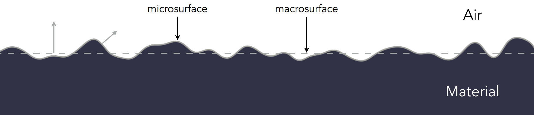
Microsurface is used to describe microfacet surfaces
Macrosurface is used to describe the underlying smooth surface (as represented by a
Shape, or otherObjectin our framework for homework).
The microfacet-based BRDF models work by statistically modeling the scattering of light from a large collection of microfacets.
If we assume that the differential area
and it is the aggregate behavior of these microfacets that determines the observed scattering.
The two main components of microfacet models are:
A representation of the distribution of facets, and
A BRDF for individual microfacets.
Perfect Mirror Reflection
most commonly used
Specular Transmission
useful for modeling many translucent materials
The Oren-Nayar Model
treats microfacets as Lambertian reflectors
Three important geometric effects to consider with Microfacet Reflection Models:
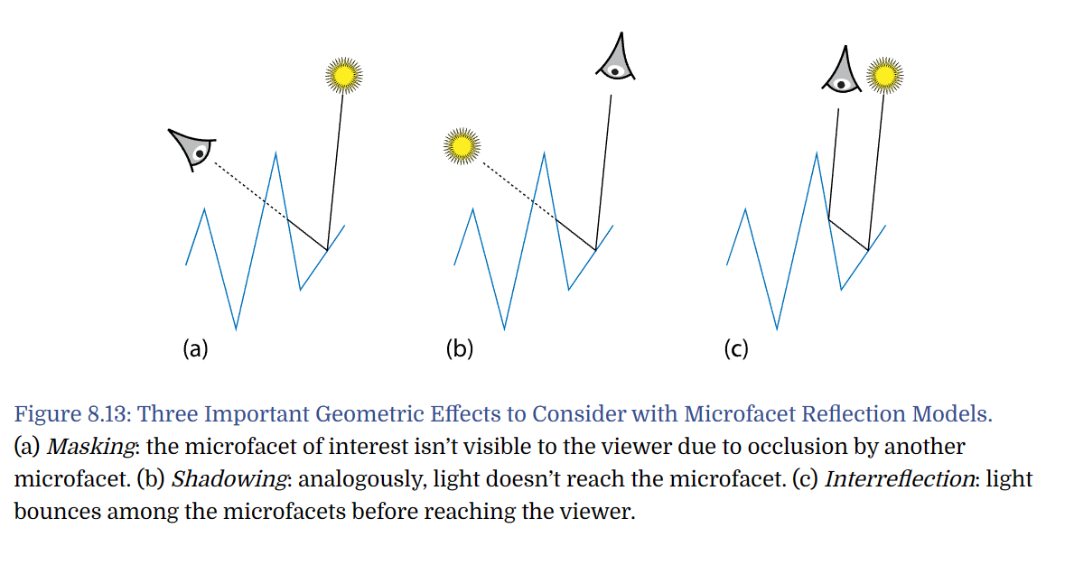
Masking
Microfacet is occluded by another facet
Shadowing
Microfacet may lie in the shadow of a neighboring microfacet
Interreflection
Cause a microfacet to reflect more light than predicted by the amount of direct illumination and the low-level microfacet BRDF
Oren-Nayar Diffuse Reflection
Idea: Real-world objects do not exhibit perfect Lambertian reflection.
Rough surfaces generally appear brighter as the illumination direction approaches the viewing direction.
Describe rough surfaces by V-shaped microfacets, which is
Described by a spherical Gaussian distribution with a single parameter
Interreflections: Only consider the neighboring microfacet
Approximation:
where if
Microfacet Distribution Functions
One important characteristics of a microfacet surface is represented by the distribution function pbrt, microfacet distribution functions are defined in the same BSDF coordinate system as BxDFs. As such,
a perfectly smooth surface could be describe by a delta distribution that was non-zero only when
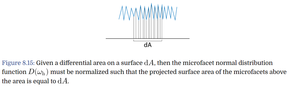
Microfacet distribution functions must be
Normalized: Given a differential area of the microsurface,
Beckmann Distribution
A widely used microfacet distribution function based on a Gaussian distribution of microfacet slops is due to Beckmann and Spizzichino.
The traditional definition of the Beckmann-Spizzichino model is
where if
RMS: Root Mean Square
The anisotropic microfacet distribution function is
Note that the original isotropic variant falls out when
When programming, the algorithm directly translates the above equation, but pay special attention to the following issues:
Infinity value of
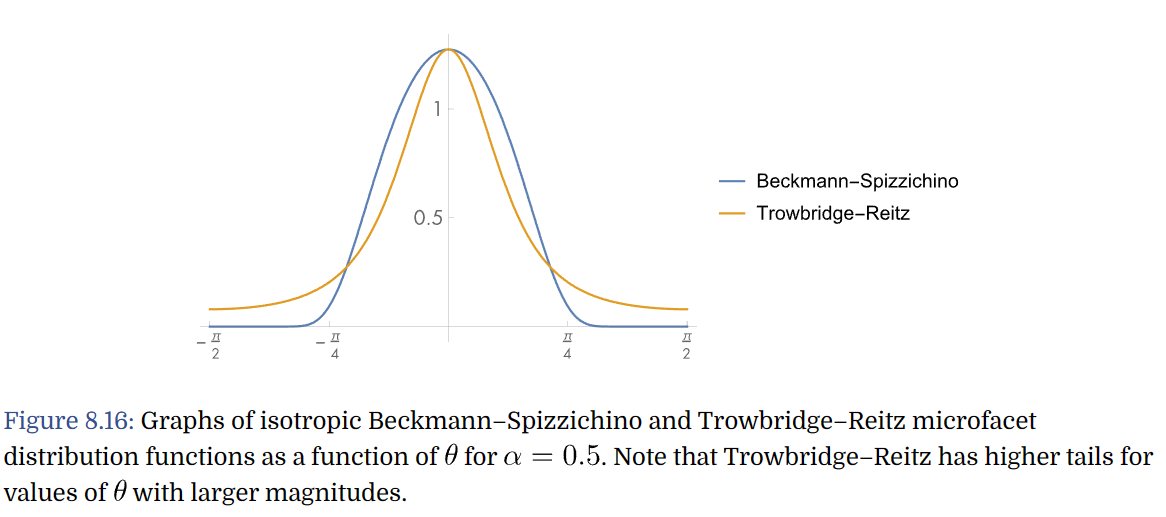
Trowbridge-Reitz Distribution
Anisotropic variant given by
In comparison to the Beckmann-Spizzichino model,
It has higher tails - it falls off to zero more slowly for directions far from the surface normal.
This characteristic matches the properties of many real-world surfaces well
Usually, we specify
Masking and Shadowing
Smith's Masking-Shadowing Function: Some microfacets will be invisible from a given viewing or illumination direction because,
They are back-facing
Some of the forward-facing microfacet area will be hidden due to being shadowed by back-facing microfacets.
This is described by
which gives the fraction of microfacets with normal
Note that
Normalization Constraint: A differential area
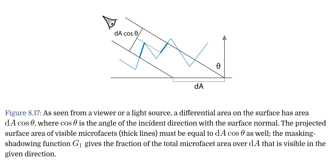
Compute
We can thus alternatively write the masking-shadowing function as the ratio of visible microfacets area to total forward-facing microfacet area:
Shadowing-masking functions are traditionally expressed in terms of an auxiliary function
After some algebra we have
Specifying
If we assume that there is no correlation between the heights of nearby points on the microsurface, then it's possible to find a unique
For many microfacet models, a closed-form expression can be found.
Although this isn't true in reality, the resulting
Beckmann-Spizzichino: Under the assumption of no such correlation, we have
where
In
pbrt, a rational polynomial approximation is used, to avoid callingstd::erf()andstd::exp()which are fairly expensive to evaluate.
Computing the interpolated
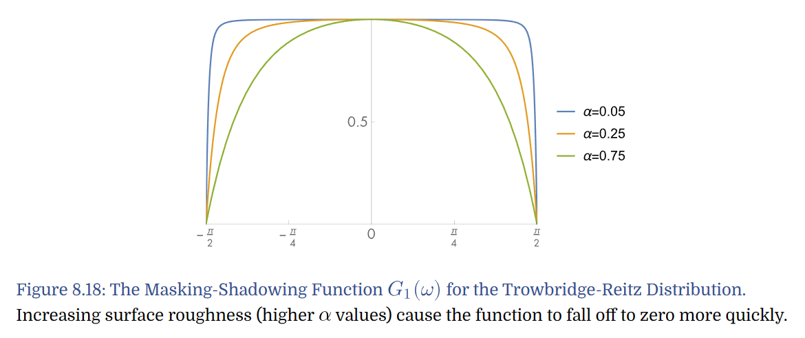
The function is close to one over much of the domain, but falls to zero at grazing angles.
Increasing surface roughness causes the function to fall off more quickly.
Computing
If we assume that the probability of a microfacet being visible from both directions is the probability that it is visible from each direction independently, then we have
In practice,
This often underestimates
The closer together the
A more accurate model can be derived, assuming that microfacet visibility is more likely the higher up a given point on a microfacet is. This assumption leads to the model
The Torrance-Sparrow Model
For very detailed derivation, refer to the PBR book. Basically, we assume that individual microfacets are perfectly specular, and therefore only those that have the direction of their normals matched with the orientation of